 Acad
AcadHow to Make a Study Area Map for Your Thesis or Paper
Learning how to make a study area map is the first cartographic hurdle nearly every thesis and research paper puts in front of you: the opening figure that tells a reviewer exactly where your work happened. A good one nests your site inside its region and country, orients the reader with a north arrow and graticule, and states scale honestly. This guide walks through the required elements, the projection mistake that silently breaks scale bars, and how to build the whole figure in Python without wrestling inset alignment by hand.
What a study area map actually needs to do
A study area map (also called a locator map or site map) answers one question for your reader: where did this research take place? It is not a results map, it is the orienting figure that comes before your data. The most common failure is showing a tightly cropped site with no wider context, forcing readers who don't know your country to guess what they are looking at.
The fix is nesting. A strong study area map for a thesis shows two or three scales at once: the country (so anyone can place it), the region or province (mid-scale context), and the site itself (your actual boundary or sampling points). This cascade is why the classic layout pairs a small country inset in a corner with a larger, detailed panel of the site.
If you remember one thing, remember this: a location map for a research paper is judged on whether a stranger to your region can find your site in about five seconds. Every element below serves that single goal, and anything that does not serve it is decoration you can cut.
The required-elements checklist
Reviewers and cartography style guides converge on a short list of elements. Treat the table below as a pre-submission checklist. The last column shows what AcadGIS does by default, so you can see which items are handled for you and which still need a human decision.
| Element | Why it matters | AcadGIS default |
|---|---|---|
| Locator / inset | Nests the site in its region and country so unfamiliar readers can place it | Auto-generated from the cascade of steps (country to region to site) |
| Study-site highlight | Draws the eye to the actual area of interest, not the whole frame | Final step highlighted; controllable via highlight= |
| North arrow | States orientation; expected whenever north is not obviously up | north_arrow=True (on by default) |
| Scale bar | Lets readers judge distance; must reflect a projected CRS to be honest | scale_bar=True (on by default) |
| Graticule | Lat/lon grid gives an absolute geographic reference | graticule enabled in study-area templates |
| Coordinate system | Honest distance and shape depend on a suitable projection | Reprojected to a locally appropriate CRS automatically |
| Legend / labels | Names the regions and features your text refers to | legend=True; labels optional per step |
Step 1 - Get boundaries and pick a projection
Every study area map starts with administrative boundaries. The two free, citable sources are GADM (detailed national and sub-national units) and Natural Earth (cleaner, generalized boundaries that are ideal for small insets). For orientation you might layer in OpenStreetMap tiles or a satellite basemap. In a manual workflow you load these as shapefiles or GeoPackages in GeoPandas or QGIS.
The projection decision matters more than beginners expect. Raw GADM data ships in unprojected latitude/longitude (EPSG:4326). Draw a scale bar on that and it quietly lies, because a degree of longitude is roughly 111 km at the equator but only about 55 km at 60 degrees north. Before you measure anything, reproject to a suitable projected CRS such as the local UTM zone or a national grid. AcadGIS applies a locally appropriate projection for you, but if you build the figure by hand in GeoPandas, do it explicitly with .to_crs() before adding a scale bar.
import acadgis as agis

# Load a country and one sub-national level (Bangladesh, India, Iraq and the USA ship offline)
bd = agis.load_boundaries("Bangladesh", level="district")
agis.plot(bd, title="Districts of Bangladesh", graticule=True)
agis.show()
Step 2 - Build the locator cascade
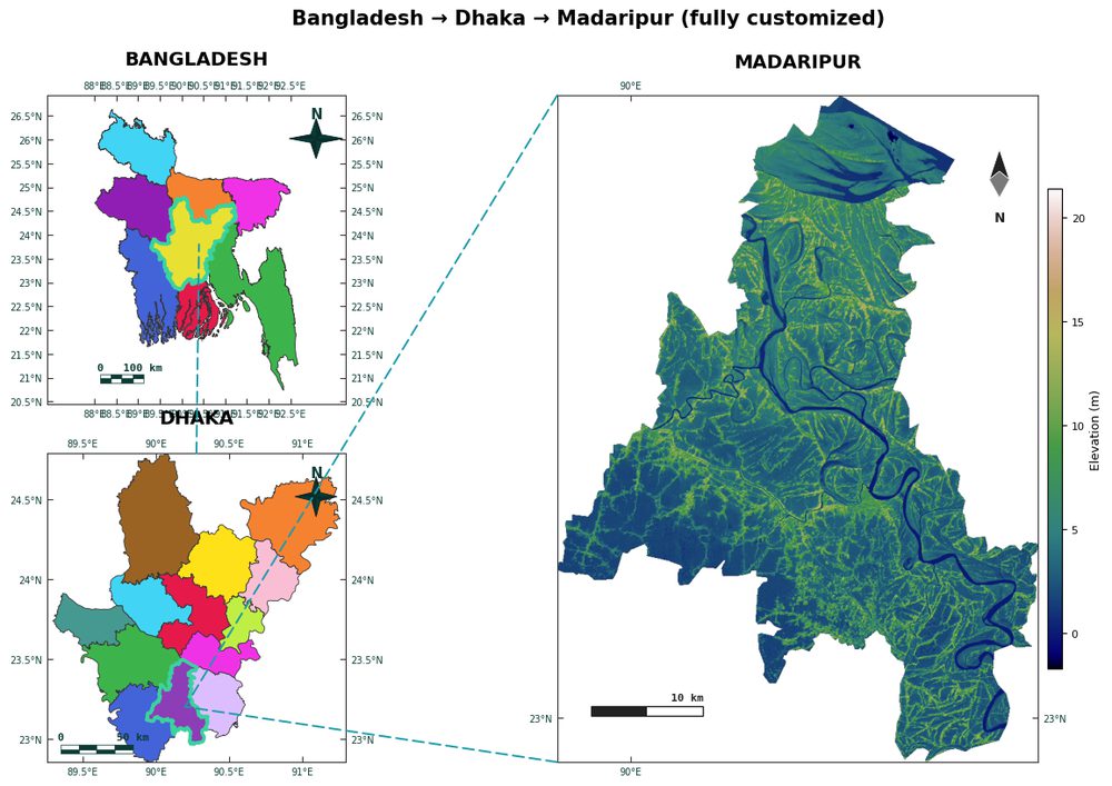
The heart of the figure is the nested cascade: country to region to site. Building this by hand means clipping boundaries at each level, aligning inset axes, and drawing connector boxes, which is tedious but entirely possible in GeoPandas or QGIS's print layout. AcadGIS collapses it into one call. The study_area() function takes an ordered list of steps and produces the whole cascade with the final step highlighted.
import acadgis as agis

fig = agis.study_area(
    "Bangladesh",
    steps=[("division", "Dhaka"), ("district", "Madaripur")],
    template="cascade",
    rivers=True,
    labels=True,
)
agis.save("madaripur_study_area.png", dpi=300)
If you prefer an object-oriented style, or want to reuse the same context across several sites, the StudyArea builder reads more fluently and is easy to parameterize in a loop.
import acadgis as agis

sa = (agis.StudyArea("India", context_level="state")
         .zoom_into("Uttarakhand", detail_level="district"))
fig = sa.figure(suptitle="Study Area: Uttarakhand, India")
agis.save("uttarakhand_study_area.png", dpi=300)
For a no-code web version of this cascade, the study area map generator and the locator map generator produce the same nested layout from dropdowns, which is handy for a quick draft before you commit to a scripted figure.
Step 3 - Add orientation: north arrow, scale bar, graticule
These three elements are what turn a picture of a shape into a map. A north arrow is only strictly required when north is not at the top, but reviewers expect one regardless. A scale bar is only meaningful on a projected map, so it depends directly on the CRS choice from Step 1. A graticule, the faint grid of latitude and longitude lines, gives an absolute reference and is especially valued in earth-science and ecology venues where a reader may want to note exact coordinates.
In a manual pipeline these come from add-ons: matplotlib-scalebar for the bar, hand-drawn arrows or plugins for orientation in QGIS, and gridline helpers for the graticule. In AcadGIS they are parameters on plot() and are on by default, so the honest work becomes deciding when to turn them off rather than scrambling to bolt them on at the end.
import acadgis as agis

bd = agis.load_boundaries("Bangladesh", level="district")
agis.plot(bd, highlight="Madaripur", north_arrow=True,
          scale_bar=True, graticule=True, title="Study Area")
agis.show()
Step 4 - Honest polish and export
Once the structure is right, the remaining choices are about clarity, not decoration. Keep the inset small and unobtrusive so it frames the site without competing with it. Label only the places your text actually references; an over-labeled map is harder to read than a sparse one. Choose a muted, colorblind-safe palette for context polygons so your highlighted site is the obvious focal point. Add rivers or terrain only if they are relevant to the study, and skip them when they are just visual noise.
Export at 300 DPI or higher for print, and prefer a vector or high-resolution raster so text and hairlines stay crisp when the page is reduced to column width. AcadGIS's agis.save("fig.png", dpi=300) handles this; in a manual workflow, set the DPI in matplotlib's savefig or export at high resolution from QGIS. For thesis figures specifically, the thesis map maker presets sizing and margins to common dissertation page dimensions so the figure drops into your template without rescaling.
When to use AcadGIS versus GeoPandas or QGIS
Be honest with yourself about the trade-off. QGIS gives you total manual control and is the right tool when your map is unusual or you need pixel-level layout tweaks. GeoPandas (with mapclassify for classification and folium for interactive web maps) is ideal when the study area map is one step inside a larger scripted analysis and you want full transparency over every layer.
AcadGIS is aimed squarely at the common case: a researcher who needs a correct, reproducible study area map in Python and does not want to hand-code inset alignment, reprojection, and scale-bar math on every new site. It rests on the same open data (GADM, Natural Earth) and the same engine (matplotlib and GeoPandas underneath), so nothing is locked away and you can drop down to the raw axes whenever you need to. When a whole set of sites needs identical styling, pairing the study area map generator with a simple loop over StudyArea keeps every figure in the series consistent.
Frequently asked questions
What is a study area map?
A study area map is the orienting figure that shows where research took place, nesting the study site inside its wider region and country. It typically includes a locator inset, a north arrow, a scale bar, and a graticule, and it appears near the start of a thesis or paper before any results maps.
How do I make a study area map in Python?
The fastest route is a dedicated library like AcadGIS, where study_area() or the StudyArea builder produces the full country-to-site cascade in one call with a north arrow, scale bar, and graticule on by default. You can also assemble one manually with GeoPandas for boundaries, mapclassify for any classification, and matplotlib for the layout, using GADM or Natural Earth data.
Where can I get free administrative boundaries for the map?
GADM provides detailed national and sub-national administrative boundaries, and Natural Earth offers cleaner generalized boundaries that work well for small insets. Both are free and citable; AcadGIS bundles Bangladesh, Iraq, India and the USA offline and downloads other countries by name.
Do I need a north arrow and scale bar on a study area map?
Yes, for most academic venues a scale bar and a north arrow are expected, and a graticule is strongly encouraged. The one caveat is that a scale bar is only meaningful on a projected map, so reproject from raw latitude/longitude to a suitable projected CRS such as the local UTM zone before adding one.
What is the difference between a study area map and a locator map?
The terms overlap heavily and are often used interchangeably. In practice a locator map emphasizes the inset that pinpoints a site within a larger area, while a study area map is the complete figure, the locator inset plus the detailed site panel with orientation elements, that opens a thesis or paper.
Can I make a consistent study area map for several sites?
Yes; because the StudyArea builder is just an object you configure, you can loop over a list of regions and call figure() for each to guarantee identical styling. This is the reliable way to produce a matched research-area series where every figure shares the same palette, projection, and layout.